What are Expected Points?
In a previous article I discussed expected goals (or xG) and how they can be used to provide a quantifiable measurement of a game’s progression. Extending this framework, and doing a bit of math, we can calculate the points a team could have expected to win based on their xG. This metric is known as expected points (xPts).
Calculating xPts
As any expected value, xPts can be calculated according to the formula:
xPts = (win probability * amount for winning) + (loss probability * amount for losing)
Because in football we have a third option – drawing – the formula changes as follows:
xPts = (win probability * points for winning) + (draw probability * points for drawing) + (loss probability * points for losing)
Plugging in the numbers for the points for winning/drawing/losing, the formula changes to:
xPts = (win probability * 3.0) + (draw probability * 1.0) + (loss probability * 0.0)
The last term can be discarded, since it will always amount to 0, so the final xPts formula is:
xPts = (win probability * 3.0) + (draw probability * 1.0)
Now that we’ve established how to calculate it, the question then arises – how do you determine the win/loss/draw probabilities?
Simulating a Game Using Monte Carlo Simulations
First of all, what are Monte Carlo Simulations (MCS)? MCS are algorithms used to “model the probability of different outcomes in a process that cannot easily be predicted due to the intervention of random variables”1 They are used routinely and extensively in “finance, engineering, supply chain, and science.”1
Now that we’ve established what MCS are, how can we use them to predict the probability of a given event (win/draw/loss) in a football game? Simply put, we can simulate a game thousands of times using the same conditions on the pitch (in this case, xG), to see how the game could have played out given the initial conditions.
We can do this in two different ways: we can use Microsoft Excel or we can write our own code. Since there are a lot of good tutorials on how to do MCS with Excel (here, here, and here), I won’t dwell on it, but rather focus on discussing how I wrote such a simulator in Python. To exemplify it, we will look at the first game of this season: Brentford – Arsenal.
Setup
The game was played on August 13, 2021, at the Brentford Community Stadium. The final score was 2-0 for Brentford, but the xG story is different: according to fbref.com/StatsBomb, Brentford’s xG was 1.3, while Arsenal’s was 1.4. So, were Brentford lucky to win? Did Arsenal deserve a draw? Let’s find out!
Code Overview
Here is the backbone of the code I wrote, which you can find on my GitHub page (freely downloadable):
- First, we need to input the home and away teams with respective xGs.
- We then need to define a number of simulations – for speed, I chose 20,000 simulations. You can go as high as you want, but that will take a longer time to complete. If you go lower, the sampling will likely not be exhaustive enough.
- Once we have this info, we need to define the type of distribution our simulations will model. It has been shown that football games are Poisson processes (see also here, and here), although that has been debated (see also here). What is a Poisson process you ask? It is a model where the average time between events is known, but the exact timing of events is random. Each team scoring is a separate Poisson process, so there will be two independent Poisson distributions being calculated, using each team’s xG as our input variable to generate these distributions.
- In each simulation, we determine the predicted goals scored by the home and away teams, the score margin, and we keep track of how many wins, draws and losses the home and away teams have.
- At the end of the 20,000 simulations, we calculate the statistics and see what the win/draw/loss probabilities are, and we calculate the expected points. We can also determine what the likeliest score is, and for this we calculate the score matrix.
This is how the workflow above looks like in code if we consider Brentford vs. Arsenal:

Results
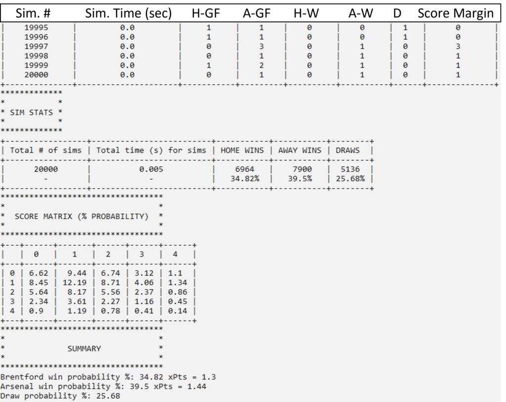
The simulation results show us that if the game had been played 20,000 times, Brentford would have won 6964 times (34.8%), Arsenal would have won 7900 times (39.5%), and a draw would have occurred 5136 times (25.7%). The expected points from these probabilities would be:
xPtsBrentford = (0.348 * 3.0) + (0.257 * 1.0) = 1.301
xPtsArsenal = (0.395 * 3.0) + (0.257 * 1.0) = 1.442
Looking at the score matrix, we can see that the likeliest score to occur is 1-1 (12.2%), whereas a 2-0 win for Brentford had a 5.6% probability of occurring. With all this info in hand, we can say that both Arsenal and Brentford had very similar chances of winning, and a 2-0 Brentford victory was not outside the realm of possibility.
What to Expect in Part II
xPts can be used to calculate a league table based on performance rather than results. Of course, this performance comes from one story of the game (i.e., xG), and should not be taken as Gospel. It does however give a good idea of whether teams are over/underperforming, and where they should be in the table if the universe was solely governed by xG.
In addition, as mentioned in my xG model comparison model, different xGs would impact the simulations and will give you different xPts. Thus, we will have a look at different models, including Understat, FiveThirtyEight, and the xPts simulated using my simulator and the fbref/StatsBomb xG values, and see how these models differ between each other.
I will also describe an xPts model that is not dependent on xG, but rather on more traditional statistical metrics that are not as esoteric as xG. Since I’m still developing it and collecting data, it might be a short while until Part II is published.
References
- https://www.investopedia.com/terms/m/montecarlosimulation.asp
Last Updated
[ratemypost]
[ratemypost-result]