xG Model Comparison

What is Expected Goals – or xG?

Briefly put, xG allows the assessment of how many goals a team could have expected to score given the quality and quantity of chances they had during a game. We’ve all been in the boat of “We played better but couldn’t convert our chances” or “We played much better than the other team, how did we lose?” By quantifying these chances, we can try and explain whether a team really deserved to win or if it was just a good ol’ smash’n’grab.

How is xG calculated?

There are multiple analytics companies and websites (Opta, StatsBomb, Understat, Smartodds, etc.) that have built up databases of hundreds of thousands of shots from tens of different leagues over multiple seasons and the related data: type of shot, shot angle, position on the pitch, distance to goal, relative defender position, etc. This data is fed into algorithms based on machine learning (ML), which come up with different probabilities for a given shot. The probabilities of all shots attempted in a game for each team are then added up. This represents the xG for each team.

Similar Yet Different

As described above, xG models are based on statistical & historical shot data. They differ in the algorithm used to build them, as well as in the quality/diversity/sheer amount of data used. Naturally, there will be variance between models trying to describe the same variable. The question here is – how large is this variance? Below find the xG values for all 20 teams in the PL so far this season from three different models – StatsBomb, Opta, and Understat. The xG values in this analysis do not incorporate penalties or own goals.

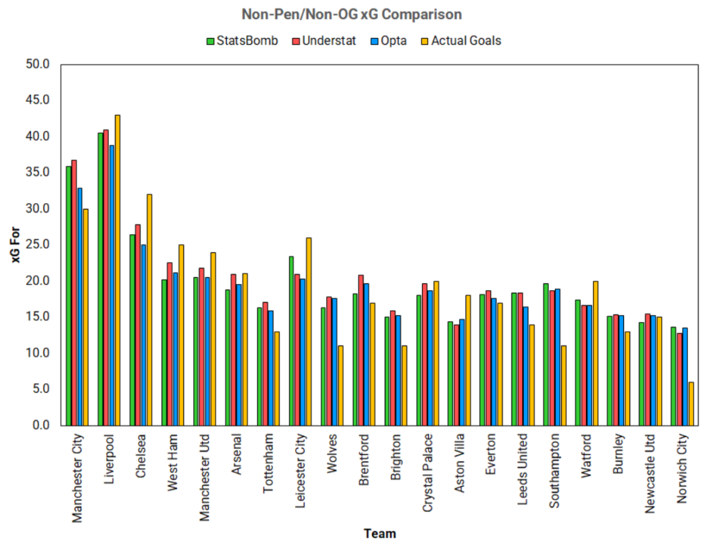
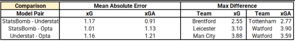
This is a busy graph so let’s deconstruct a bit. First, notice how the values between the three models are similar yet quite a bit different. In fact, the mean absolute error between each pair of models is ~1 xG, for both goals scored and conceded. However, the maximum difference between them is quite high, with the highest xG difference being between Understat and Opta (Man City, 3.88) and the highest xGA being between StatsBomb and Opta (Watford, 3.90).

Going back to the graph, it’s quite clear that all 3 models think that City should have scored more goals than they have so far. On the other hand, Liverpool, Chelsea, West Ham, Man U, Leicester, even Watford, have all outperformed their expected goal tally. Norwich City on the other hand, are incredibly poor at finishing their chances, as well as Wolves and Southampton. Let’s move onto xGA.

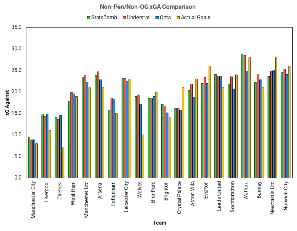
Both Liverpool and City are outperforming their xGA and are conceding far fewer goals than expected. On the other hand, Crystal Palace are conceding far more than they would be expected to be. Again, notice how the values differ quite a bit between models (i.e., Watford, Tottenham).

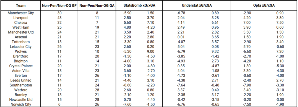
While the models show similar trends for under/overperforming teams, the differences between the values are not insignificant. Thus, I thought of averaging the values for each team across models, computing standard deviations, and then comparing to the actual goals scored/conceded.

Composite vs. Individual

Below find the values for the composite xG model based on the averages of the three models considered above.

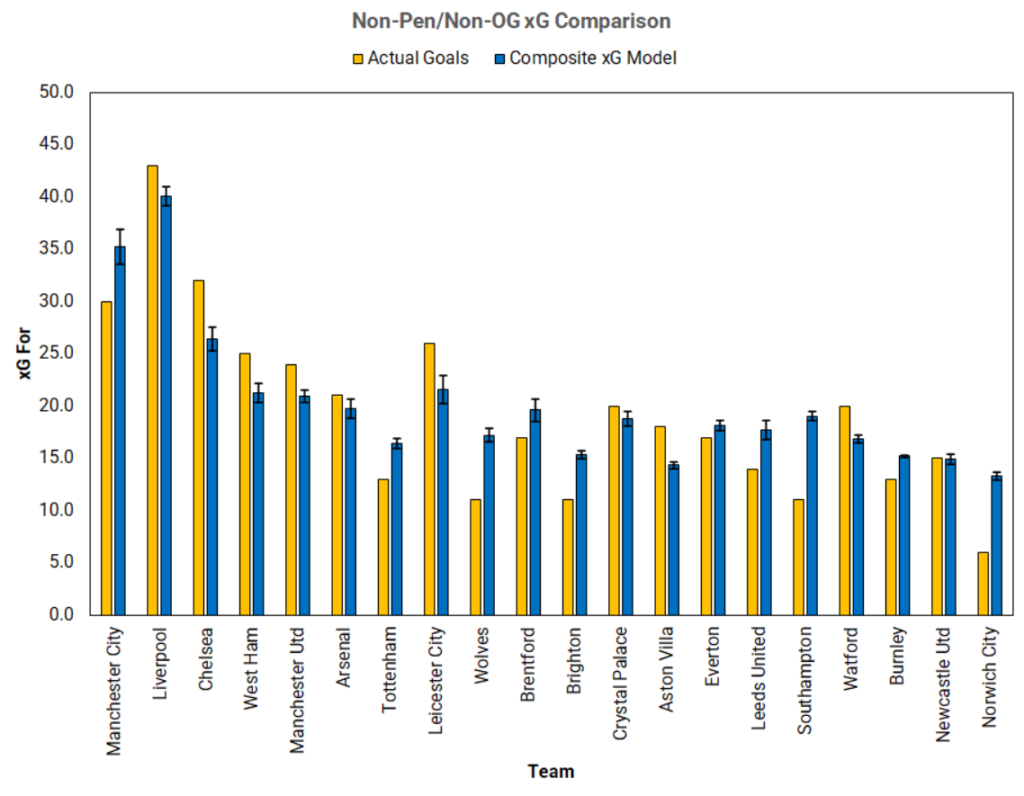
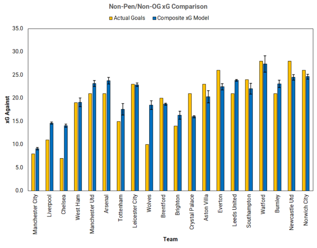
With these composite values we can now get a better idea of much teams over/underperform this season in terms of goals scored/conceded.

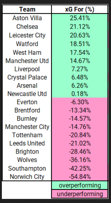
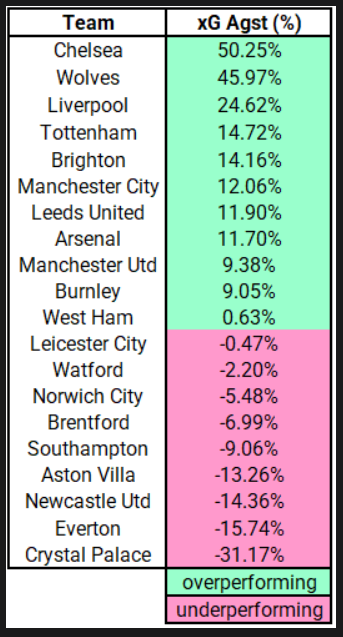
Based on these values, Villa have outperformed their xG For by almost 25%. On the other hand, Wolves, Southampton and Norwich are severely underperforming in terms of goals scored based on their xG data. In terms of xG against, Chelsea have conceded 50% fewer goals than their xG against suggests, while Palace have conceded 31% more goals than their xG against suggests.

Conclusion

All xG data is based on models and approximations. Moreover, it would be a fallacy to think that xG represents the full story of a game. At best, xG presents a story of the game. Different models will give you different results, so it is important to consider this when describing the performance of a team and whether they deserved to win or not. Averaging across models and computing standard deviations is likely to give you a better overview than using one model alone.

Last Updated

[ratemypost]

[ratemypost-result]