Pythagoras and Football
As a natural follow-up to the first part of this series, I wanted to see if I could build a model that takes into account well-known metrics that are different from xG (i.e., total shooting rate, goals scored/allowed, passes under pressure, pitch tilt etc). After collecting data and formulating all sorts of hypotheses in my mind that used different parameter combinations, I came across something fantastic that would make my job much easier – the Pythagorean Expectation.
The Pythagorean Expectation (PythExp) was devised by Bill James as a way to determine how many games a baseball team should have won based on the numbers of runs scored and allowed. This in turn allows one to identify the teams that are over/underperforming by comparing PythExp to the actual win percentage (win%). This is very similar to expected points models in football, where one compares points rather than win%s.
The PythExp formula itself is very simple:
PythExp = (Runs Scored)2 / (Runs Scored2 + Runs Allowed2)
The reason the formula works is two-fold: first, teams win baseball games as a result of their quality (runs scored vs. runs allowed). This of course follows in football as well, although there are xG arguments that a team should have scored more/less than they actually did (more on this later). For example, if a team scores 25 runs and allows 20, their measure of quality would be 25/20 = 1.250 (and vice versa for their opponent, 20/25 = 0.800). The probability of winning for the first team would be 1.25 / (1.25 + 0.80) = 0.609 = 60.9%. This of course is the exact same thing as writing:

which leads to the original PythExp formula above. This relationship holds true for any number of runs scored/allowed.
Second, baseball, as football, involves a non-negligible amount of chance, which allows teams to fluctuate around the games they should have won but didn’t and those they shouldn’t have won but did. This in turn allows for the exponent to be very close to 2. This relationship does not hold true for basketball, where the exponent is close to 14.
The PythExp formula was derived empirically by James, but further development by numerous statisticians resulted in slightly more accurate exponents (1.83 being used for example by baseball-reference.com, the baseball counterpart to fbref.com). I will leave the exponents as 2, as they are easier to understand in reference to the Pythagorean Theorem.
Does the PythExp Formula Hold for Football?
My hypothesis was the following: because baseball and football roughly follow the same two rules described above, the PythExp formula should yield accurate results for football. To verify this hypothesis, I assembled and curated a data set of league standings from the Big 5 Leagues, starting with the 2017/18 season. The reason I did not go further back was because fbref only started collecting xG data from this season onward.
Even so, I had 392 data points to work with, which was quite enough for what I wanted to do. Once I had the standard stats + xG data, I calculated the Pythagorean Expectation as follows:
PythExp_Gls = (GF)2 / (GF2 + GA2)
Next, I calculated the win% for every data point. Because football has an extra type of result compared to baseball, the win% is calculated as:
win% = (1 * #wins + 0.5* #draws) / # of games
Once this was done, I plotted the values across all five leagues in a least-squares regression plot.
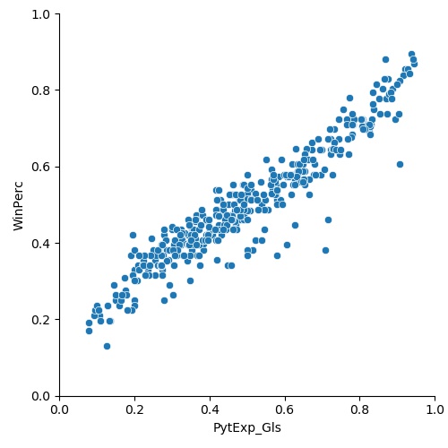
The plot above shows a beautiful correlation between the PythExp_Gls and the win%. In fact, the R2 coefficient is 0.90, which means that the Pythagorean Expectation value can explain 90% of the variance in winning percentages. In addition, I calculated some statistical parameters to ensure the correlation was statistically significant:

The p test (P >|t|) is a way to ensure results are statistically significant, and the threshold for significance is usually taken as 0.05. In our case, that threshold is smaller (0.000,..), so we conclude that our correlation is not because of chance.
Once I established this, I wanted to see what the correlation was between the PythExp based on the StatsBomb (fbref) xG and win%:
PythExp_xG_SB = (xGF_SB)2 / (xGF_SB2 + xGA_SB2)

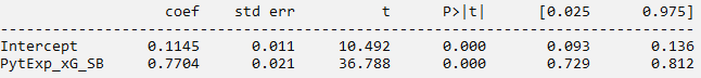
It is obvious that the scatter is wider compared to the one above, and this is also captured in the R2 coefficient (0.78). Just as was the case above, the correlation is statistically significant, with a p value < 0.05.
Is Two Better than One?
As I mentioned above, there are proponents of a purely xG model when looking at teams under/overperforming. I believe that while xG data provides lots of useful information, the goals scored/allowed should not be disregarded. So, I created a Pythagorean Expectation value based on the average of goals scored and xGF and the goals allowed and xGA.
AdjGlsF = (GF + xGF_SB)/2 ; AdjGlsA = (GA + xGA_SB)/2
PytExp_Gls_SB_Combo = (AdjGlsF)2 / (AdjGlsF2 + AdjGlsA2)
I plotted this against the win%:
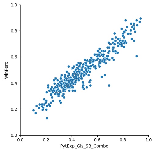

The plot is now tighter again towards the center, the R2 coefficient is 0.89, and the p value is < 0.05. The correlation coefficient is almost identical to that of only using goals, but the advantage of a hybrid goal/xG model is that it encapsulate information held in both values, as opposed to one or the other.
Note: I did these exact same steps with xG data from Understat and the results are similar, so I’m only showing the fbref data.
Predicting Points
So far we’ve established that a hybrid goal/xG model is good at predicting win%, but our main objective was to predict points. So, how do we go about doing that? First, we need to normalize the points data in the 0-1 range so that we’re working on the same scales as PythExp. The normalization is done as follows across all 392 data points:
NormalizedPoints = (pts – min_pts_in_set))/(max_pts_in_set – min_pts_in_set)
Once this is done, we plot it against the PythExp_Gls, PythExp_xG_SB, and PythExp_Gls_SB_Combo.

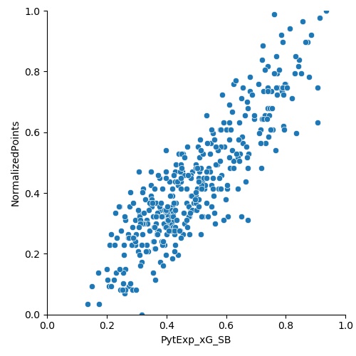
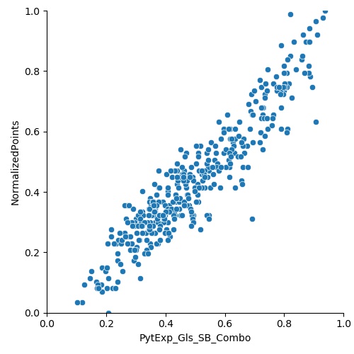
The R2 coefficients are 0.89, 0.77, and 0.88, with all three p values < 0.05. We have now determined that there is an excellent correlation between the PythExp (both goals and goals combined with xG) and the normalized points. Using the parameters from the linear regression for the PythExp_Gls (intercept = 0.0008, coefficient = 0.8846) and PythExp_Gls_SB_Combo (intercept = -0.0643, coefficient = 1.0082), we can finally predict points in two different ways with the formulas:
NormalizedPoints = 0.8846 x PythExp_Gls + 0.0008
NormalizedPoints = 1.0082 x PythExp_Gls_SB_Combo – 0.0643
Once we have the normalized points, we can un-normalize them using the formula:
NormalizedPoints x (max_pts_in_set – min_pts_in_set) + min_pts_in_set = xPts
Premier League Season 2021-22
Using the coefficients determined above along with the normalized points, PythExp_Gls and PythExp_Gls_SB_Combo we can get the points each team should have. For completeness purposes, I have also curated and collected expected points data from FiveThirtyEight, Understat, and Monte Carlo simulations using the fbref xG data. While FiveThirtyEight do pre-match predictions, their model also calculates xPts, so I wanted to see what the differences are between all xPts predictions.
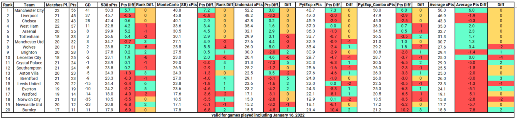
First, there are a few interesting aspects to these predictions that I would like to discuss. All 5 models agree that Manchester City have between 4-7 points more than they should, meaning that they are currently overperforming compared to their offensive/defensive output. Next, all 5 models agree that Burnley are severely underperforming, same as Newcastle and Brentford. Interestingly, 4/5 models (while the 538 is very close to 0) say that Crystal Palace should have between 5-7 points more than they currently do, and should be a few places up in the table.
As a last step, I averaged the points across all five models to come up with one, all encompassing model that could hopefully describe the PL situation this season.
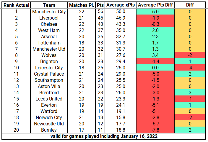
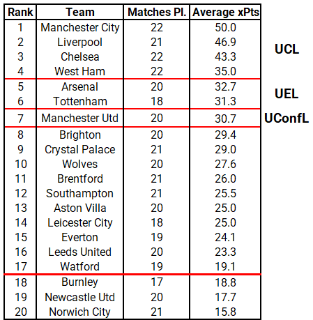
The average points model shows us that the top 7 teams are exactly where they are supposed to be. City are currently edging out games they should probably draw (see games vs Chelsea & Arsenal), while Wolves are punching above their weight by 3.4 points. On the other hand, Crystal Palace should be two places higher up in the table with 5 more points added to their tally, whereas Burnley are severely underperforming by almost 8 points, followed by Newcastle with 6 points. Below find the ranking given by the average expected points model:
Concluding Thoughts and Remarks
Debates between fans on whether a team should be higher or lower in the league table are a tale as old as time. I believe bringing these sorts stats in football is a fun way to expose fans to a world different than that of opinions, and to maybe have some data to back claims up. Of course, all the models I presented above come with associated errors, some higher than others. They are also not to be taken as Gospel. Football is played on goals, and what matters at the end of the day is the actual league table. But that doesn’t mean expected points models don’t make for good discussion!
Last Published
[ratemypost]
[ratemypost-result]